NLP/NLU Series: Clustering Linkedin Profiles
Overview:
This notebook shows off how I built a simple model that leans heavily on the power of Sentence Transformers BERT to pull out lots of features. The model is pretty simple because it’s based on K-means, but there’s a ton of space to jazz it up and make it more complex. Basically, the algorithm I’ve got going here is a rock-solid starting point for the job of grouping similar LinkedIn profiles together.
Here’s a brief rundown of the algorithm:
- Extract BERT embeddings for sentences or textual data.
- Concat them into single vector.
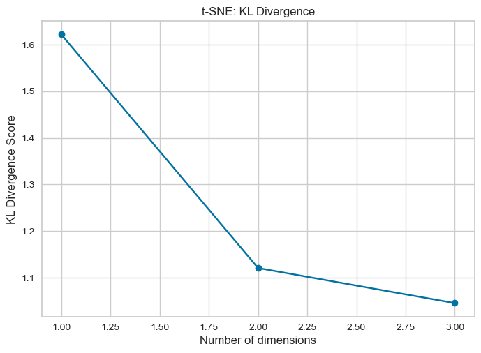
- Use t-SNE to find optimal number of dimensions that explains the data.
- Reduce dimensionality using PCA.
- Find the optimal number of clusters from K-means by using distortion metric.
- Fit reduced data to optimal number of clusters extracted from the step above.
- Project Extracted clusters to original data.
from utils import *
from modeling_utils import *
import pandas as pd
import numpy as np
from sklearn.cluster import KMeans
from yellowbrick.cluster import KElbowVisualizer
from sklearn.preprocessing import StandardScaler

import warnings
warnings.filterwarnings('ignore')
Utils, helper functions for visualizations:
def plot_missing_data(df):

    missing_data = df.isnull().sum() / len(df) * 100
    missing_data = missing_data[missing_data != 0]
    missing_data.sort_values(ascending=False, inplace=True)

    plt.figure(figsize=(6, 6))
    sns.barplot(y=missing_data.index, x=missing_data)
    plt.title('Percentage of Missing Data by Feature')
    plt.xlabel('Percentage Missing (%)')
    plt.ylabel('Features')
    plt.show()

def visualize_normalized_histogram(df, column, top_n=100, figsize=(6, 20)):

    value_counts = df[column].value_counts().nlargest(top_n)
    value_counts_normalized = (value_counts / len(df) * 100).sort_values(
        ascending=True)

    colors = plt.cm.get_cmap('tab20')(np.arange(top_n))[::-1]

    plt.figure(figsize=figsize)
    plt.barh(value_counts_normalized.index, value_counts_normalized.values, color=colors)
    plt.ylabel(column)
    plt.xlabel('Percentage')
    plt.title(f'Normalized Value Counts Histogram of {column} (Top {top_n})')
    plt.xticks(rotation=0)
    plt.show()

def visualize_top_15_category_histogram(data,
                                        category_column,
                                        cluster_column,
                                        top,
                                        title,
                                        width,
                                        height):

    top_n_categories = data[category_column].value_counts().nlargest(top).index.tolist()
    filtered_data = data[data[category_column].isin(top_n_categories)]

    fig, ax = plt.subplots(
        figsize=(width / 80, height / 80))
    sns.histplot(data=filtered_data,
                      x=category_column,
                      hue=cluster_column,
                      multiple="stack",
                      ax=ax)

    ax.set_title(title)
    for label in ax.get_xticklabels():
        label.set_rotation(90)
        label.set_fontsize(10)
    plt.show()


def get_latest_dates(df):
    df['sort_key'] = np.where(df['date_to'] == 0, df['date_from'], df['date_to'])
    df = df.sort_values(['member_id', 'sort_key'], ascending=[True, False])
    latest_dates = df.groupby('member_id').first().reset_index()
    latest_dates = latest_dates.drop(columns=['sort_key'])

    return latest_dates
Utils, helper functions for preprocessing:
def transform_experience_dates(experience):
    def transform_date_format(date_value):
        try:
            if isinstance(date_value, int) or date_value.isdigit():
                return str(date_value)  # Return the integer or numeric string as is
            else:
                date_string = str(date_value)
                date_object = datetime.strptime(date_string, "%b-%y")
                return date_object.strftime("%Y-%m")  # Format with year and month only
        except ValueError:
            return None

    def extract_year(value):
        if isinstance(value, str):
            pattern = r'\b(\d{4})\b'  # Regular expression pattern to match a four-digit year
            match = re.search(pattern, value)
            if match:
                return str(match.group(1))
        return None

    experience['transformed_date_from'] = experience['date_from'].apply(transform_date_format)
    experience['transformed_date_to'] = experience['date_to'].apply(transform_date_format)

    experience.loc[experience['transformed_date_from'].isnull(), 'transformed_date_from'] = experience.loc[
        experience['transformed_date_from'].isnull(), 'date_from'].apply(extract_year)
    experience.loc[experience['transformed_date_to'].isnull(), 'transformed_date_to'] = experience.loc[
        experience['transformed_date_to'].isnull(), 'date_to'].apply(extract_year)

    experience['transformed_date_from'] = experience['transformed_date_from'].str.replace(r'-\d{2}$', '', regex=True)
    experience['transformed_date_to'] = experience['transformed_date_to'].str.replace(r'-\d{2}$', '', regex=True)

    return experience
Utils, helper functions for modeling:
def find_optimal_dimensions_tsne(data, perplexity_range):
    dims = []
    scores = []

    max_dim = min(3, data.shape[1] - 1)

    for dim in range(1, max_dim + 1):
        if dim > len(perplexity_range):
            break

        tsne = TSNE(n_components=dim)
        embeddings = tsne.fit_transform(data)

        dims.append(dim)
        scores.append(tsne.kl_divergence_)

    # Plot the KL divergence scores
    plt.plot(dims, scores, marker='o')
    plt.xlabel('Number of dimensions')
    plt.ylabel('KL Divergence Score')
    plt.title('t-SNE: KL Divergence')
    plt.show()

    optimal_dim_index = scores.index(min(scores))
    optimal_dimensions = dims[optimal_dim_index]

    return optimal_dimensions


def reduce_dimensionality_with_pca(data, components):
    pca = PCA(n_components=components)
    reduced_data = pca.fit_transform(data)
    return reduced_data


def fit_kmeans_and_evaluate(data,
                            n_clusters=4,
                            n_init=100,
                            max_iter=400,
                            init='k-means++',
                            random_state=42):
    data_copy = data.copy()

    kmeans_model = KMeans(n_clusters=n_clusters,
                          n_init=n_init,
                          max_iter=max_iter,
                          init=init,
                          random_state=random_state)

    kmeans_model.fit(data_copy)

    silhouette = silhouette_score(data_copy, kmeans_model.labels_, metric='euclidean')
    print('KMeans Scaled Silhouette Score: {}'.format(silhouette))

    labels = kmeans_model.labels_
    clusters = pd.concat([data_copy, pd.DataFrame({'cluster_scaled': labels})], axis=1)

    return clusters
Basic Employee Features:
basic_features = pd.read_csv("Clean Data/basic_features.csv")
basic_features['member_id'] = basic_features['member_id'].astype(str)
basic_features.replace("none",np.NAN,inplace=True)
Employees Education:
education = pd.read_csv("Clean Data/employees_education_cleaned.csv")
# transform member_id to string for ease of use
education["member_id"] = education["member_id"].astype(str)
education = education[education["member_id"].isin(basic_features["member_id"])]
plot_missing_data(education)
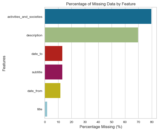
education.drop(["activities_and_societies","description"],axis=1,inplace=True)
education[["date_from","date_to"]] = education[["date_from","date_to"]].fillna(0)
education[["date_from","date_to"]] = education[["date_from","date_to"]].astype(int)
education[["title","subtitle"]] = education[["title","subtitle"]].fillna("none")
# get the latest employee education obtained per member_id:
latest_education = get_latest_dates(education)
visualize_normalized_histogram(latest_education, 'title', top_n=100)
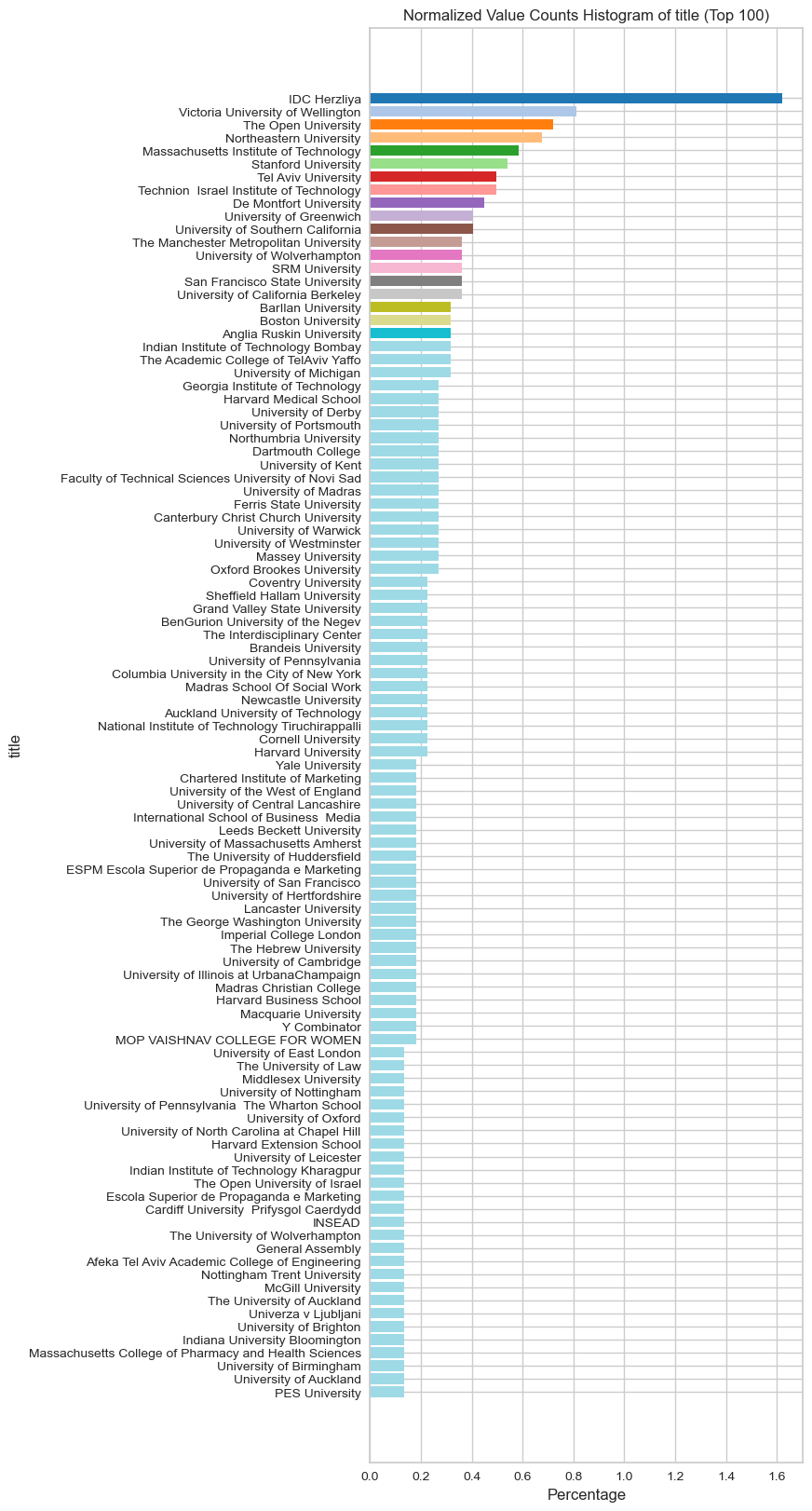
latest_education_drop_nan = latest_education.copy()
latest_education_drop_nan = latest_education_drop_nan[latest_education_drop_nan["subtitle"] != 'none']
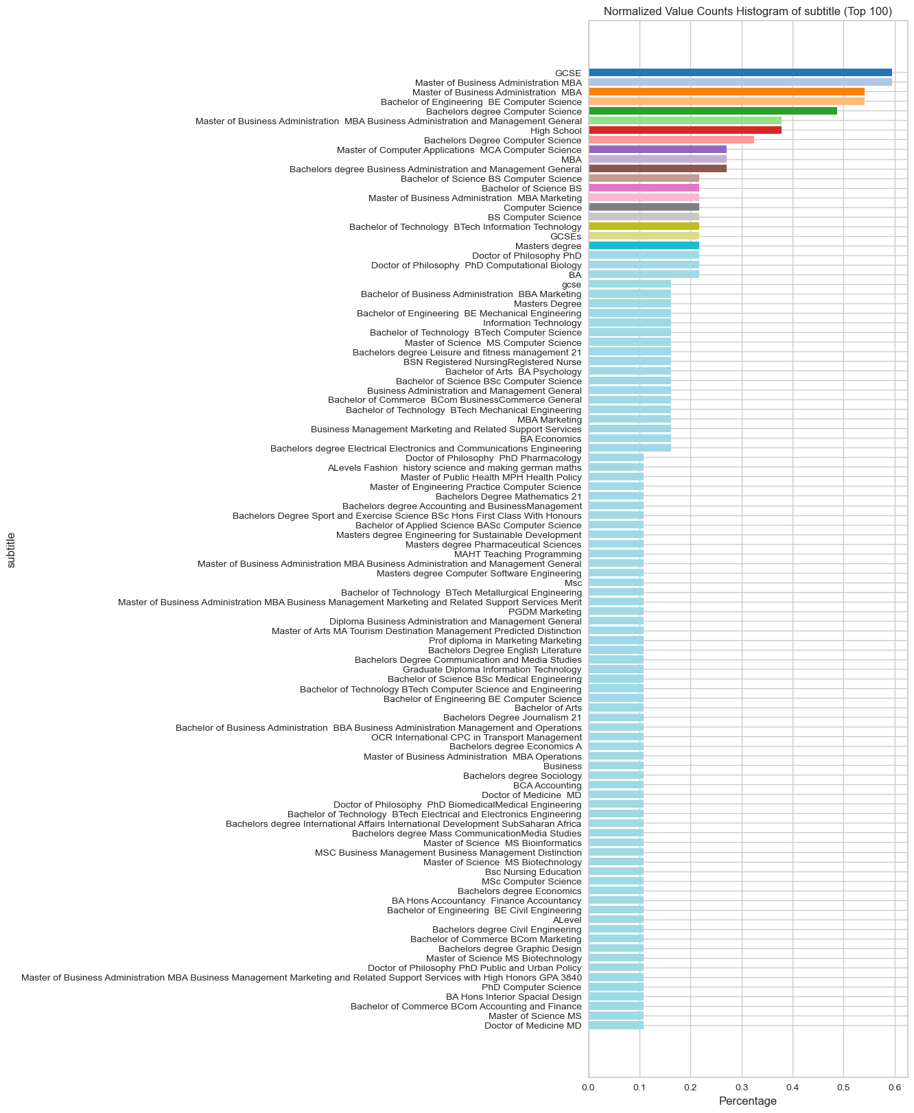
# None is causing a problem it might influence the segmentation algorithm:
visualize_normalized_histogram(latest_education_drop_nan, 'subtitle', top_n=100)
Employees Experience:
experience  = pd.read_csv("Clean Data/employees_experience_cleaned.csv")
# transform member_id to string for ease of use
experience["member_id"] = experience["member_id"].astype(str)
experience = experience[experience["member_id"].isin(experience["member_id"])]
plot_missing_data(experience)
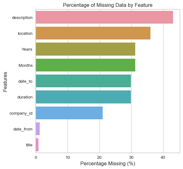
experience.drop(["description","location","Years","Months","duration","company_id"],
                 axis=1,inplace=True,
                 errors="ignore")

experience[["date_from","date_to"]] = experience[["date_from","date_to"]].fillna(0)
experience["title"] = experience["title"].fillna("none")
experience.drop_duplicates(inplace=True)
experience = transform_experience_dates(experience)
experience = experience[["member_id","title","transformed_date_from","transformed_date_to"]]
experience.rename(columns={'transformed_date_from': 'date_from',
                           'transformed_date_to': 'date_to'},inplace=True)
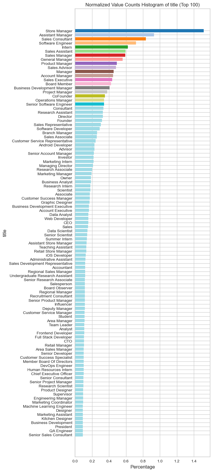
visualize_normalized_histogram(experience[experience["title"]!="none"], 'title', top_n=100)
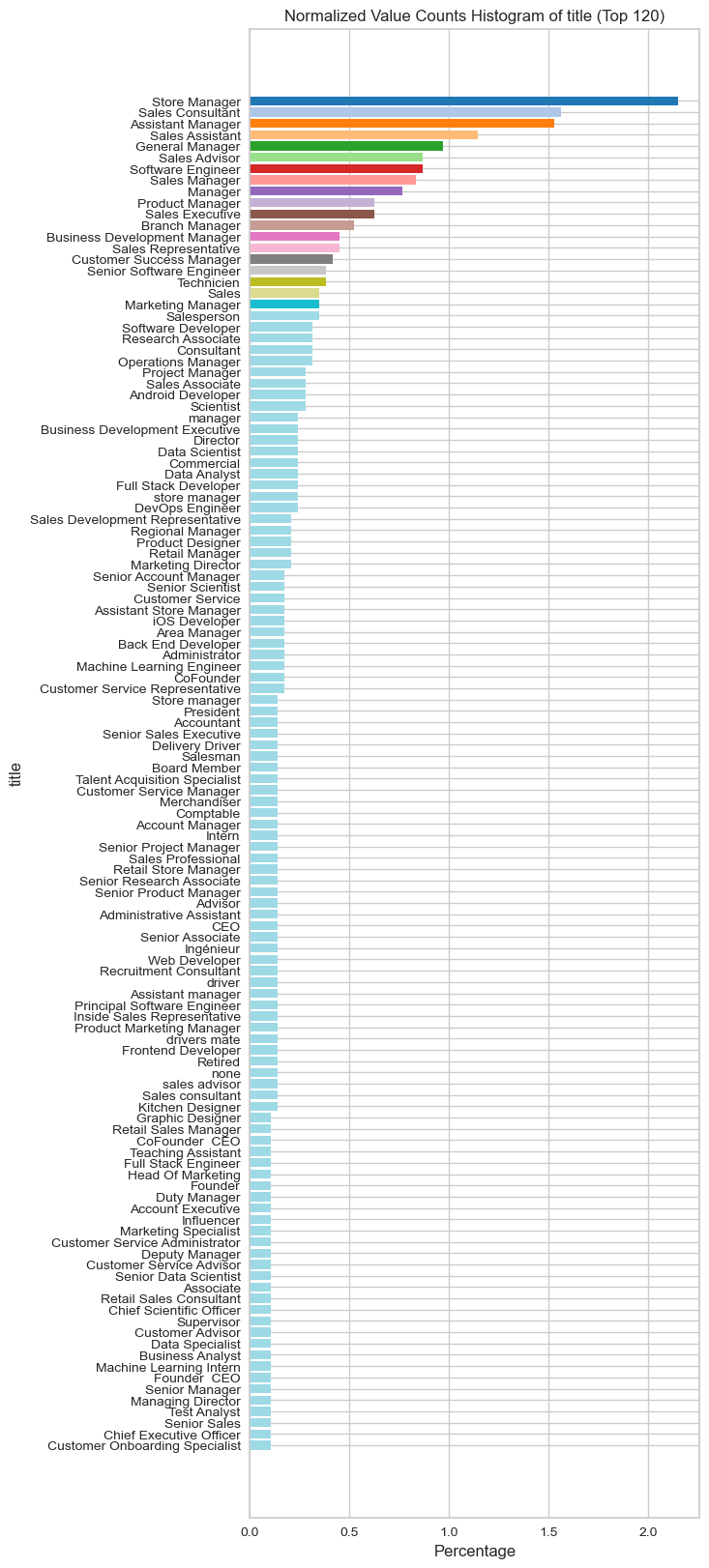
latest_experience = get_latest_dates(experience)
visualize_normalized_histogram(latest_experience, 'title', top_n=120)
Basic Features:
basic_features.isnull().sum()
member_id                   0
title                      75
location                    2
industry                 1175
summary                  1399
recommendations_count       0
country                     0
connections_count           0
experience_count            0
latitude                    0
longitude                   0
months experience        1460
number of positions      1460
number of degrees         660
years of educations       660
dtype: int64
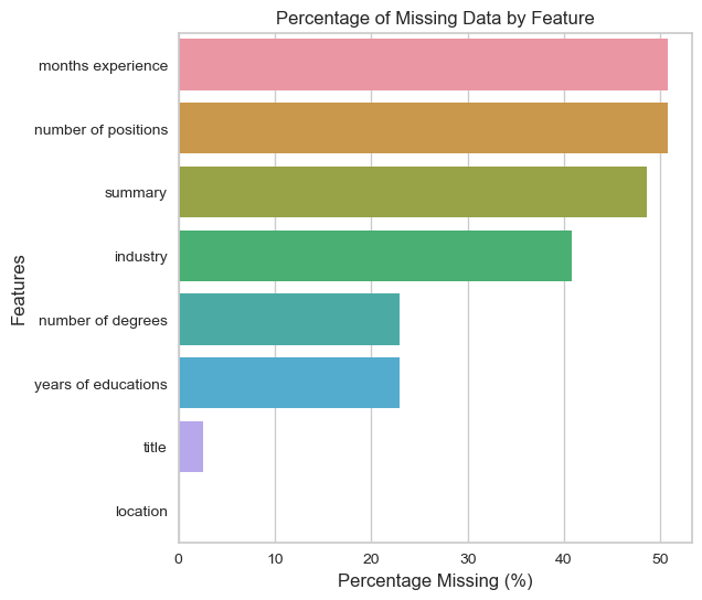
Remove columns with high percentage of missing values as they affect the results of cluster:
plot_missing_data(basic_features)
basic_features["industry"] = basic_features["industry"].fillna("other")
basic_features["title"] = basic_features["title"].fillna("other")
basic_features["location"] = basic_features["location"].fillna("unknown")
basic_features[["number of degrees","years of educations"]] = basic_features[
                                                              ["number of degrees",
                                                              "years of educations"]
                                                              ].fillna("0")
basic_features.drop(["months experience",
                     "number of positions",
                     "summary"],
                      axis=1,
                      inplace=True)
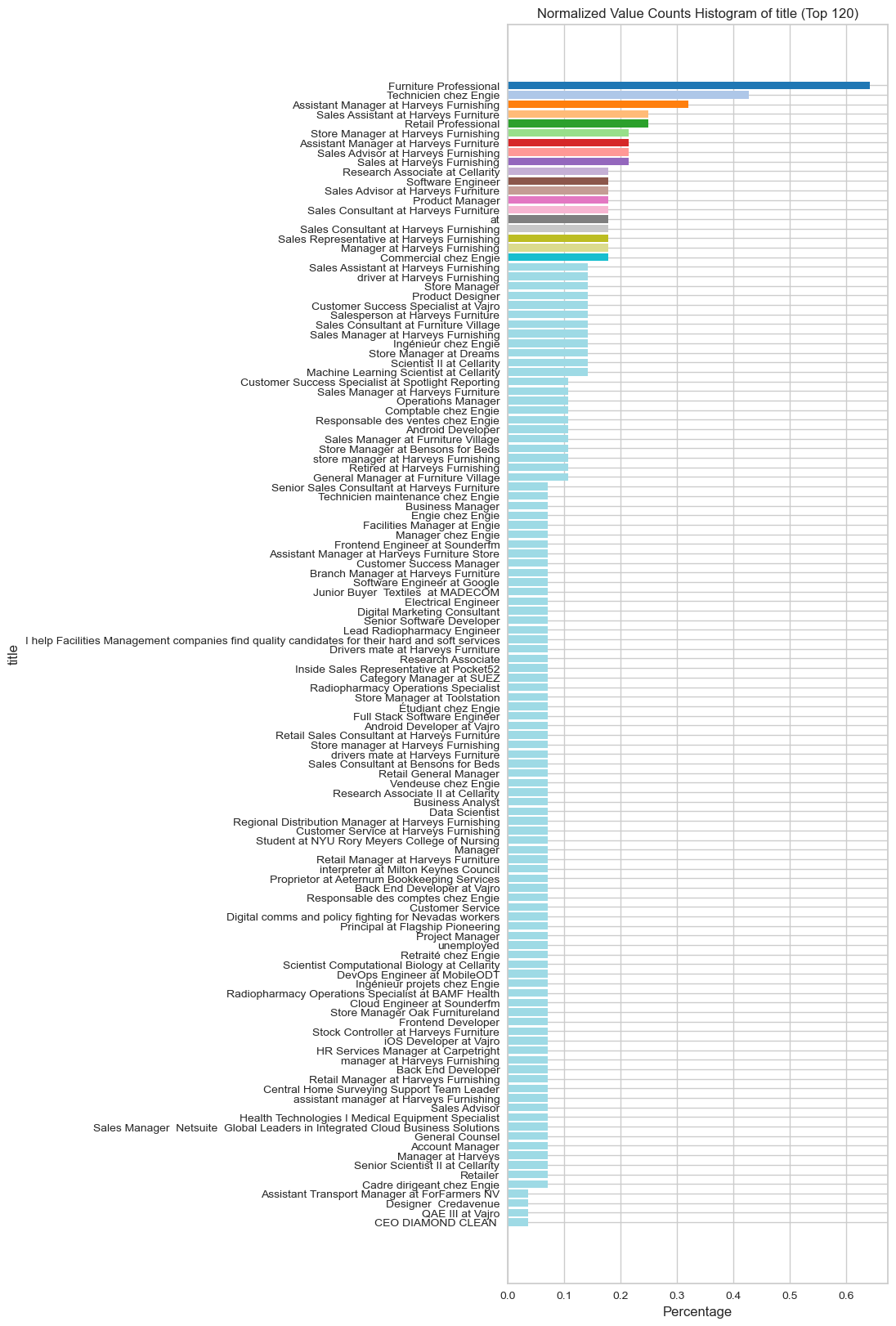
visualize_normalized_histogram(basic_features[basic_features["title"]!="other"],
                                              "title",
                                               top_n=120)
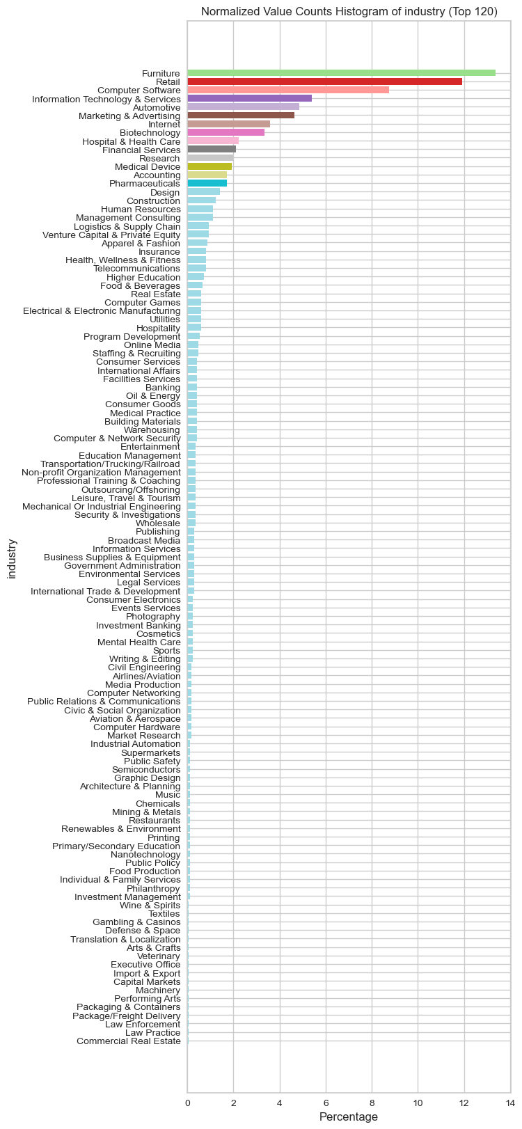
visualize_normalized_histogram(basic_features[basic_features["industry"]!="other"],"industry",top_n=120)
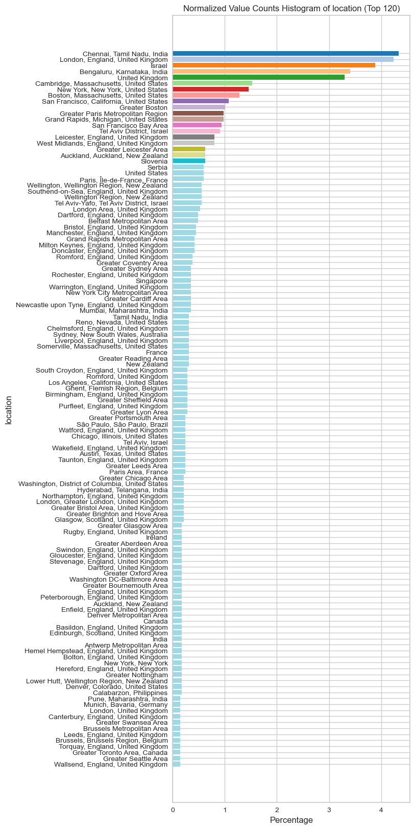
visualize_normalized_histogram(basic_features,"location",top_n=120)
Merge employees basic features, the latest education and experience:
latest_experience.drop(["date_from","date_to"],axis=1,inplace=True,errors="ignore")
latest_experience.rename(columns={"title":"experience_title"}, inplace=True)
latest_experience.head(10)
| member_id | experience_title | |
|---|---|---|
| 0 | 1000769811 | Sales Channel Advisor |
| 1 | 1001027856 | Product Development Assistant |
| 2 | 1001731893 | VP RD |
| 3 | 1002107022 | Digital Marketing Ecommerce Consultant |
| 4 | 1002900696 | Branch Manager |
| 5 | 1003503234 | Founding Shareholder |
| 6 | 1004617047 | RRH |
| 7 | 1004931912 | Senior Product Development Specialist |
| 8 | 1005561303 | Sales consultant |
| 9 | 100559115 | Marketing B2B Specialist |
latest_education.drop(["date_from","date_to"],axis=1,inplace=True,errors="ignore")
latest_education.rename(columns={"title":"education_title","subtitle":"education_subtitle"}, inplace=True)
latest_education.head(10)
| member_id | education_title | education_subtitle | |
|---|---|---|---|
| 0 | 1000769811 | University of California Santa Barbara | BA Business EconomicsPhilosophy Double Major |
| 1 | 1001027856 | British Academy of Interior Design | Postgraduate Diploma Interior Design |
| 2 | 1001731893 | The Academic College of TelAviv Yaffo | Computer Science |
| 3 | 1002107022 | Epping forest college | 2 A levels Computer studies |
| 4 | 1002900696 | bridge road adult education | OCN Psychology criminal Psychology Psychosocia... |
| 5 | 1003503234 | Lancaster University | BSc Hons in Management |
| 6 | 1004617047 | Université Paris II Assas | Master II Droit et pratique des relations du t... |
| 7 | 1004931912 | University of Michigan | Post doc Radiopharmaceutical Chemistry in Nucl... |
| 8 | 1005561303 | Rother Valley College | Btec diploma in business finance business pas... |
| 9 | 100559115 | CONMEBOL | Certified Sports Managment |
overall_features = basic_features.merge(latest_education, on='member_id', how='outer').merge(latest_experience, on='member_id', how='outer')
additional preprocessing:
string_columns = ["education_title",
                  "country",
                  "industry",
                  "location",
                  "title",
                  "education_subtitle",
                  "experience_title"]
overall_features[string_columns] = overall_features[string_columns].fillna('none')

numerical_cols = ["experience_count",
                  "connections_count",
                  "years of educations",
                  "number of degrees",
                  "recommendations_count",
                  "longitude",
                  "latitude"]
overall_features[numerical_cols] = overall_features[numerical_cols].fillna(0)
overall_features.isnull().sum()
member_id                0
title                    0
location                 0
industry                 0
recommendations_count    0
country                  0
connections_count        0
experience_count         0
latitude                 0
longitude                0
number of degrees        0
years of educations      0
education_title          0
education_subtitle       0
experience_title         0
dtype: int64
visualize_none_percentages(overall_features)
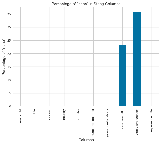
Drop rows that contain “none” as it effects the performance of Clustering:
overall_features = overall_features[~overall_features.apply(lambda row: row.astype(str).str.contains('none')).any(axis=1)]
overall_features = overall_features[~overall_features.apply(lambda row: row.astype(str).str.contains('other')).any(axis=1)]
overall_features[["title","industry","location","country","education_title","education_subtitle","experience_title"]].head(5).style.background_gradient()
| title | industry | location | country | education_title | education_subtitle | experience_title | |
|---|---|---|---|---|---|---|---|
| 4 | I Help Professionals Make Career Business Breakthroughs Coaching Consulting Personal Branding Resumes LinkedIn Profile Thought Leadership Development | Information Technology & Services | Dallas, Texas, United States | United States | Harvard University | Bachelor of Arts BA Computer Science Focus on Artificial Technology Machine Learning and Education Techology | SVP Customer Success |
| 6 | Sr Research Engineer at BAMF Health | Medical Device | Grand Rapids, Michigan, United States | United States | Grand Valley State University | Master of Science Engineering Biomedical Engineering | Image Processing Research Engineer |
| 7 | Head of New Business at Cube Online | Events Services | Sydney, New South Wales, Australia | Australia | University of the West of England | BA Hons Business Studies | APAC Hunter Manager |
| 8 | Veneer Sales Manager at Mundy Veneer Limited | Furniture | Taunton, England, United Kingdom | United Kingdom | Northumbria University | Masters Degree MSc Hons Business with Management | Project Coordinator |
| 10 | ML Genomics Datadriven biology | Computer Software | Cambridge, Massachusetts, United States | United States | Technical University of Munich | Doctor of Philosophy PhD Computational Biology | Computational Biologist |
Extract Sentence Embeddings:
### extract high dimensional embeddings using sentence transformer BERT:
title_embeddings = get_embeddings(overall_features,'title')
industry_embeddings = get_embeddings(overall_features,'industry')
location_embeddings = get_embeddings(overall_features,'location')
country_embeddings = get_embeddings(overall_features,'country')
education_title = get_embeddings(overall_features,'education_title')
education_subtitle = get_embeddings(overall_features,'education_subtitle')
experience_title = get_embeddings(overall_features,'experience_title')
Merge with simple features:
merged_embeddings = np.concatenate((
    title_embeddings,
    industry_embeddings,
    location_embeddings,
    country_embeddings,
    education_title,
    education_subtitle,
    experience_title
), axis=1)

additional_numerical_features = overall_features[[
    'recommendations_count',
    'connections_count',
    'experience_count',
    'latitude',
    'longitude',
    'member_id'
]].values

simple_features = basic_features[['recommendations_count',
                                  'connections_count',
                                  'experience_count',
                                  'latitude',
                                  'longitude', ]]

final_data = np.concatenate((merged_embeddings, additional_numerical_features), axis=1)
final_data = pd.DataFrame(final_data)


# keep a list or ordered members_ids to use later for explanations:
members_ids = final_data.iloc[:, -1].tolist()

# drop members_id, as it's not used in modeling the data, and it will
# lead to misleading results:
final_data = final_data.drop(final_data.columns[-1], axis=1)
Find Optimal Number of Components:
find_optimal_dimensions_tsne(merged_embeddings, [5,10,15,20,25,30,35,40,45,50])
Reduce Embedding Dimensionality:
reduced_merged_embeddings = reduce_dimensionality_with_pca(merged_embeddings,3)
reduced_merged_embeddings = pd.DataFrame(reduced_merged_embeddings)
reduced_merged_embeddings
| 0 | 1 | 2 | |
|---|---|---|---|
| 0 | -0.309824 | -0.357302 | 0.296566 |
| 1 | -0.611905 | -0.678734 | -0.044584 |
| 2 | 0.103592 | 0.197899 | 0.296579 |
| 3 | 0.664791 | -0.113497 | 0.114943 |
| 4 | -0.656240 | -0.552984 | 0.348519 |
| ... | ... | ... | ... |
| 1140 | 0.779930 | -0.071203 | 0.002138 |
| 1141 | 0.859704 | -0.109584 | -0.098612 |
| 1142 | -0.502135 | 0.747044 | 0.863029 |
| 1143 | 0.561427 | -0.077284 | -0.185717 |
| 1144 | -0.542131 | 0.734136 | -0.657090 |
1145 rows × 3 columns
Scale Simple Numerical Features:
scaler = StandardScaler()
scaled_data = scaler.fit_transform(simple_features)
scaled_data = pd.DataFrame(scaled_data)
Merge with Reduced Embedding Vectors:
merged_embeddings = pd.DataFrame(merged_embeddings)
all_features = pd.concat([merged_embeddings, scaled_data], axis=1)
Find optimal number of K that describes the data with the smallest distortion score:
model = KMeans(n_init=10)
visualizer = KElbowVisualizer(model, k=(2,10))
visualizer.fit(reduced_merged_embeddings)
visualizer.show()
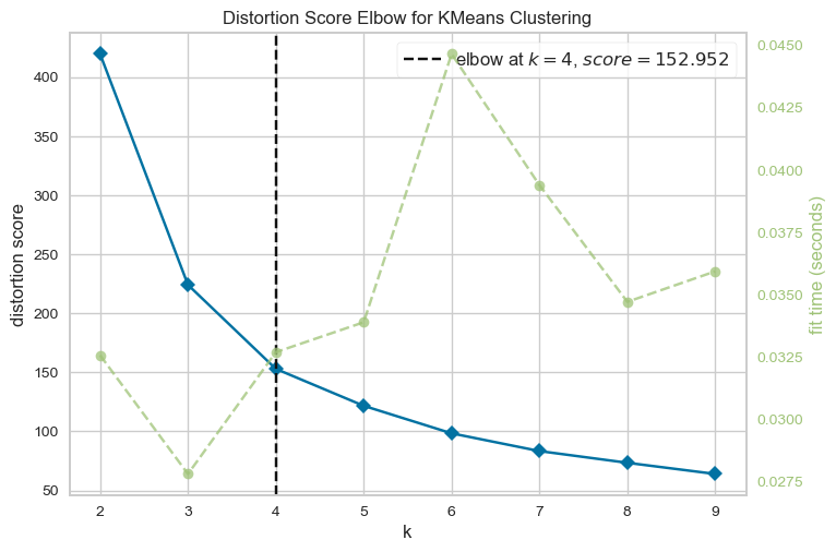
<Axes: title={'center': 'Distortion Score Elbow for KMeans Clustering'}, xlabel='k', ylabel='distortion score'>
merged_embeddings_clusters = fit_kmeans_and_evaluate(reduced_merged_embeddings,
                                                     4,
                                                     n_init=100,
                                                     max_iter=100000,
                                                     init='k-means++',
                                                     random_state=412)
KMeans Scaled Silhouette Score: 0.5201332569122314
# rename extracted clusters:
merged_embeddings_clusters = merged_embeddings_clusters.rename(columns={0:"component 1",
                                                                        1:"component 2",
                                                                        2:"component 3"})
merged_embeddings_clusters["member_id"] = members_ids
overall_features["member_id"] = overall_features["member_id"].astype(int)
merged_embeddings_clusters["member_id"] = merged_embeddings_clusters["member_id"].astype(int)
overall_results = overall_features.merge(merged_embeddings_clusters,on='member_id')
overall_results["cluster_scaled_string"] = overall_results["cluster_scaled"].astype(str)
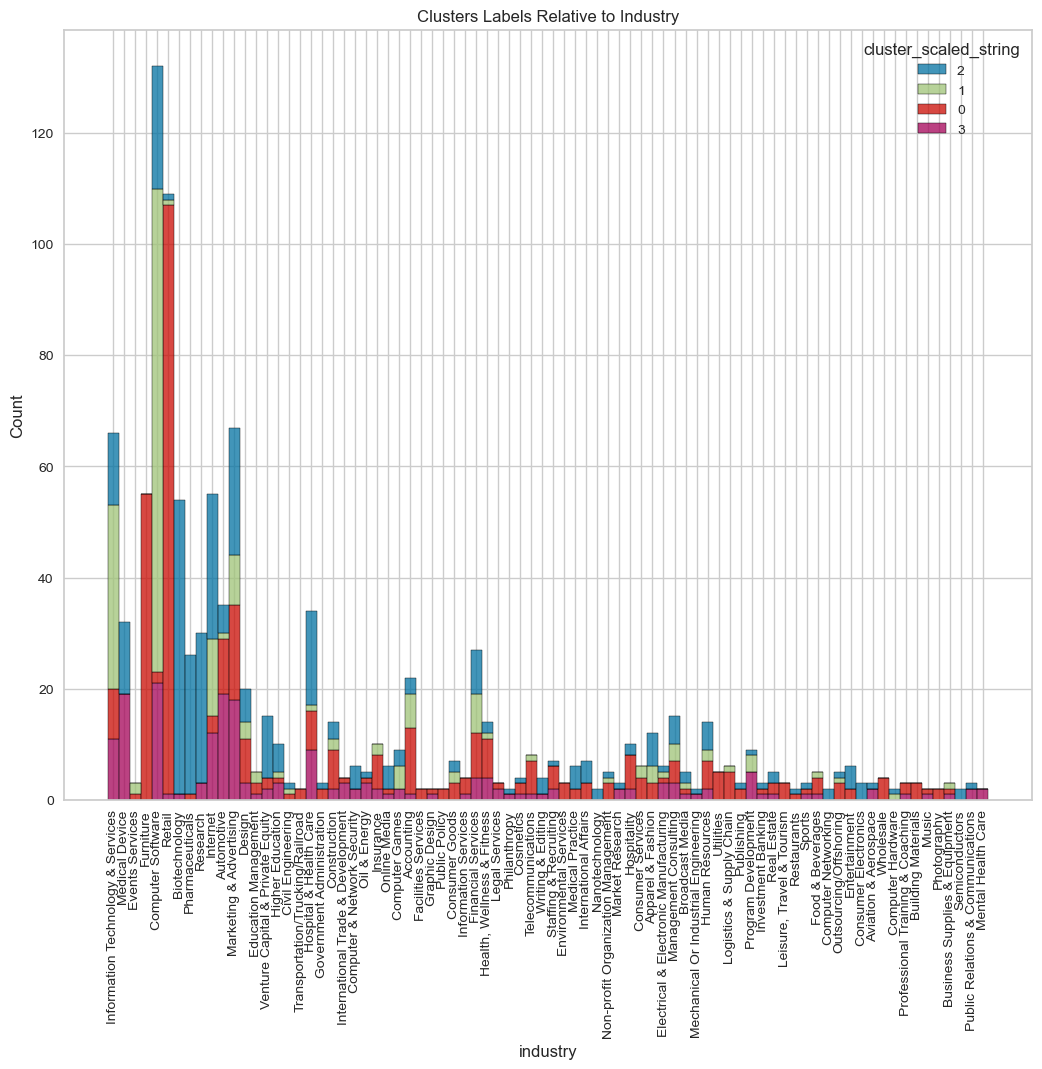
visualize_top_15_category_histogram(overall_results,
                                    category_column="industry",
                                    cluster_column="cluster_scaled_string",
                                    top=80,
                                    title="Clusters Labels Relative to Industry",
                                    width=1000,
                                    height=800
                                    )
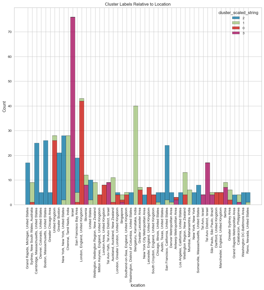
visualize_top_15_category_histogram(overall_results,
                                    category_column="location",
                                    cluster_column="cluster_scaled_string"
                                    ,top=50,
                                    title="Cluster Labels Relative to Location",
                                    width=1000,
                                    height=800
                                    )
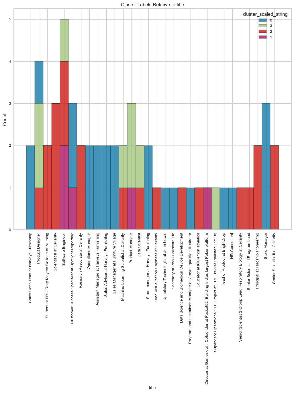
visualize_top_15_category_histogram(overall_results,
                                    category_column="title",
                                    cluster_column="cluster_scaled_string",
                                    top=30,
                                    title="Cluster Labels Relative to title",
                                    width=1000,
                                    height=800
                                    )
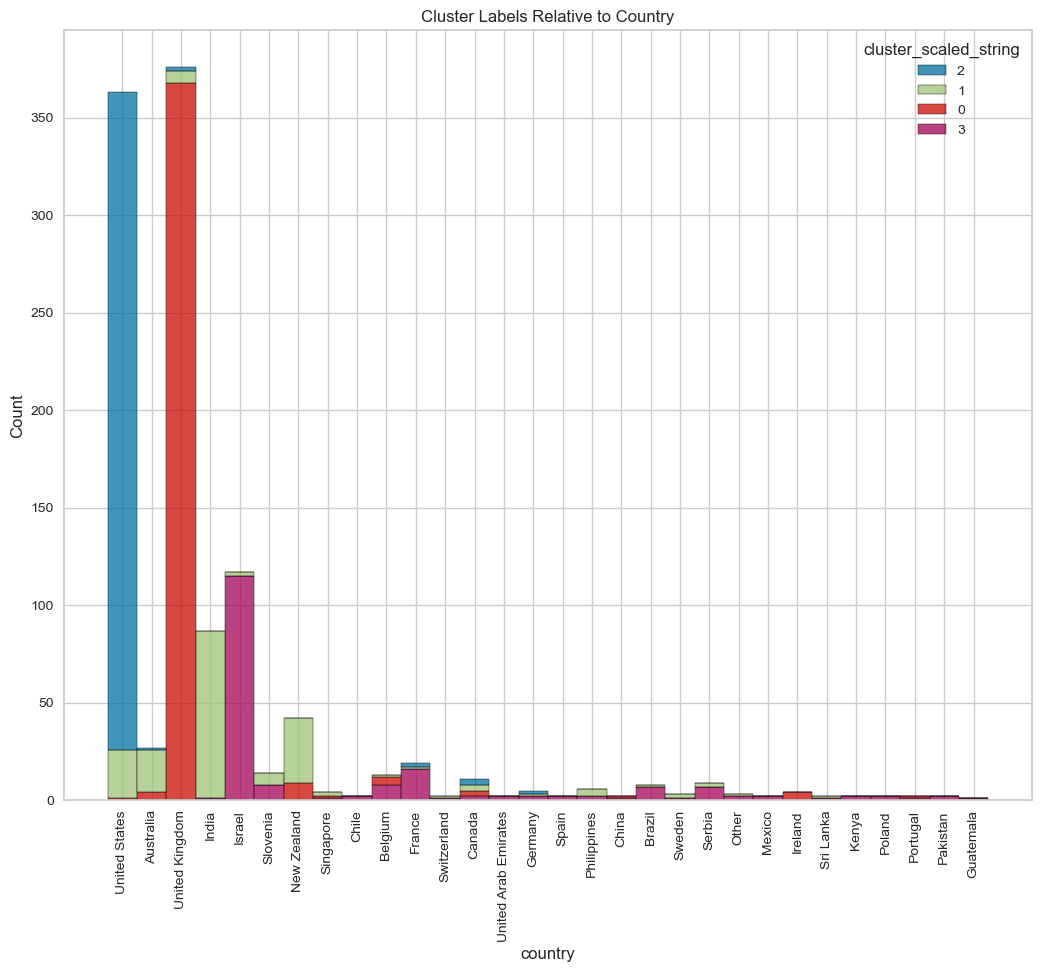
visualize_top_15_category_histogram(overall_results,
                                    category_column="country",
                                    cluster_column="cluster_scaled_string",
                                    top=30,
                                    title="Cluster Labels Relative to Country",
                                    width=1000,
                                    height=800
                                    )
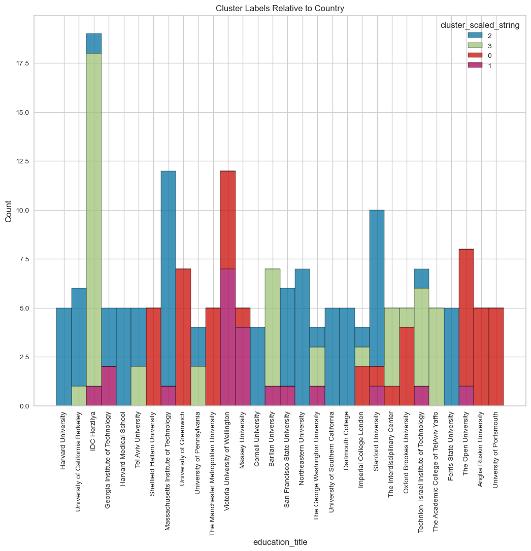
visualize_top_15_category_histogram(overall_results,
                                    category_column="education_title",
                                    cluster_column="cluster_scaled_string",
                                    top=30,
                                    title="Cluster Labels Relative to Country",
                                    width=1000,
                                    height=800
                                    )
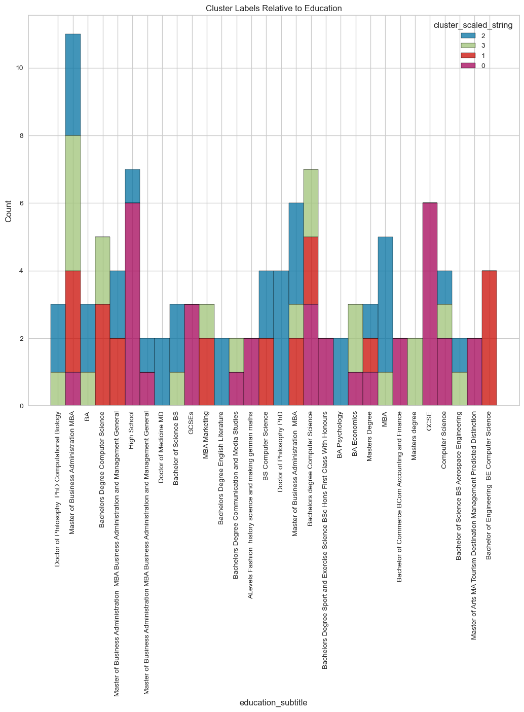
visualize_top_15_category_histogram(overall_results,
                                    category_column="education_subtitle",
                                    cluster_column="cluster_scaled_string",
                                    top=30,
                                    title="Cluster Labels Relative to Education",
                                    width=1000,
                                    height=800
                                    )
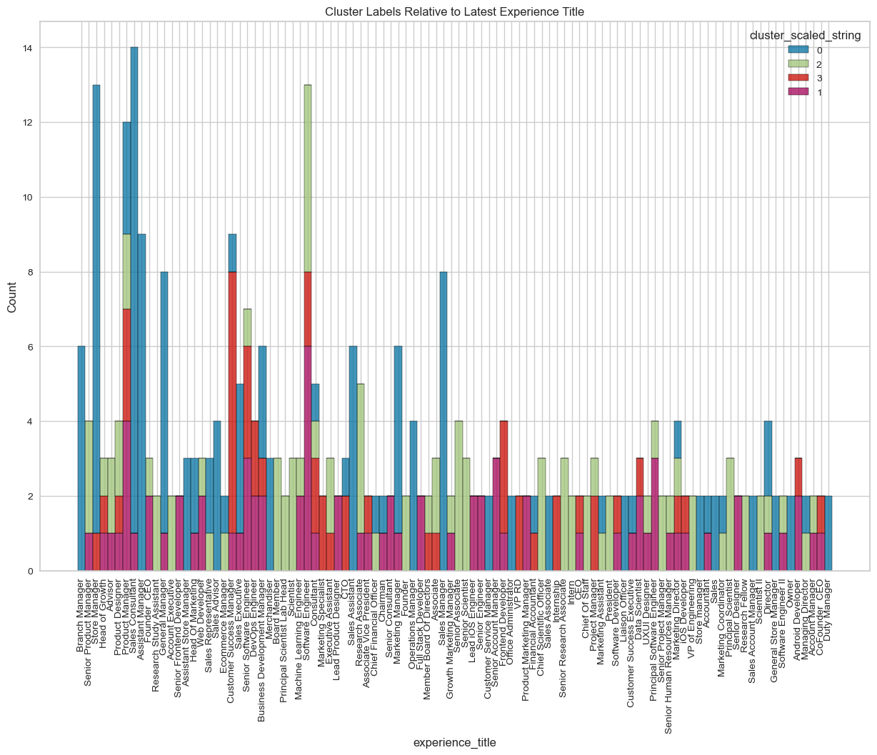
visualize_top_15_category_histogram(overall_results,
                                    category_column="experience_title",
                                    cluster_column="cluster_scaled_string",
                                    top=100,
                                    title="Cluster Labels Relative to Latest Experience Title",
                                    width=1200,
                                    height=800
                                    )
overall_results.to_csv("Clean Data/overall_results.csv",index=False)
Observations:
- By squishing together the big, complex text features, K-means did a pretty solid job. With a Distortion Score of 152 and a Silhouette Score of 0.5201, we think it’s a good place to start.
- We can probably make the clusters even better if we pull in more info like recommendations, education, and job history.
- The model seems to be pretty good at putting employees from the same industries together. Take a look at cluster 2 - it grouped retail and furniture folks together.
- In terms of where people are from, the model’s done a good job. It’s been putting places from the same country together, like Israel and its districts and cities in cluster 0, and it did the same with US cities in cluster 1. This kind of data looks like it’d work well with hierarchy-based models like HDBSCAN.
- One thing to note is that the model likes to stick all the empty values or “none” or “other” categories together, mostly because they look alike when transformed into vectors. To steer clear of this, I decided to leave them out.
- Just a heads-up that I used K-means here, which is pretty simple and can be thrown off by outliers. In the future, it could be worth making a fancier model that’s tougher against outliers.